Introduction to Computational Archaeology

Introduction to Computational Archaeology

This book is designed to help archaeologists develop foundational and applied skills in data analysis and visualization using programming languages like Python and R. Whether you are working with excavation records, environmental data, radiocarbon dates, or artifact distributions, this book will guide you through hands-on, project-based exercises grounded in real-world archaeological questions.

Who Is This Book For?

This book is intended for students, researchers, or professionals in archaeology who want to:

  • Develop essential data literacy and computational thinking
  • Use programming tools to clean, analyze, and visualize archaeological data
  • Apply statistical models to real-world excavation or survey data
  • Understand archaeological networks, typologies, and temporal trends

What Will You Learn?

Over the course of 12 chapters, you will explore topics such as:

  • Sets, relations, and structuring archaeological data in Python
  • Probability, exploratory data analysis, and Bayesian inference
  • Decision trees, feature engineering, and categorical data modeling
  • Network visualization, GIS concepts, and spatial analysis
  • Regression, hypothesis testing, Monte Carlo simulations
  • Time series analysis and forecasting in archaeological research

Why Does This Matter?

Important: Archaeology is increasingly data-driven. From spatial modeling to typological classification, today’s archaeologists must be able to work confidently with datasets, digital tools, and visualizations. This book provides the practical skills to make sense of the complex, multi-dimensional data encountered in the field, lab, and archive.

How Is the Book Structured?

Each chapter includes:

  • A clear overview of the concepts and tools covered
  • Examples relevant to archaeological fieldwork and analysis
  • Hands-on exercises using Python and R
  • A tutorial that builds toward your capstone projects
  • A short activity at the end of each section

Getting Started

🧭 Activity: Prepare Your Toolkit

To begin, please install the following tools:

  • Python 3.x – preferably with Anaconda or Jupyter Notebooks
  • R and RStudio – for Chapters 8–12
  • VS Code or another text editor for working with Python files
  • Download the example archaeological datasets provided in Chapter 1

Once your environment is set up, proceed to Chapter 1: Sets, Relations, and Data Structures in Python.

Chapter 1: Data Structure in Archaeology using Python

Chapter 1: Data Structure in Archaeology using Python

Welcome to the first chapter of Introduction to Computational Archaeology. In this chapter, we lay the groundwork for how archaeologists can use Python to represent and work with structured data. Whether you’re organizing field notes, cataloguing artifacts, or preparing data for statistical analysis, understanding how to structure and relate data is an essential first step.

What You’ll Learn

You will be introduced to the core mathematical concepts of sets, relations, and cardinality, and how these can be represented and manipulated in Python using basic data structures like lists, sets, and dictionaries. You’ll also begin creating simple visualizations to explore your data.

Why It Matters in Archaeology

Archaeological data is often complex and deeply relational — one object might be linked to multiple features, time periods, or material categories. Understanding how to express these relationships computationally allows you to organize excavation data, digitize typologies, and eventually run more advanced analyses.

Example: Imagine needing to manage a digital catalog of thousands of artifacts from multiple trench layers, each with their own attributes (e.g., material, date, condition). Sets and relations will help you efficiently structure this dataset and prepare it for analysis.

What You’ll Be Able to Do

  • Understand the basics of sets, relations, and how data is structured
  • Create and manipulate simple data structures in Python
  • Use these structures to represent archaeological information such as artifact collections, stratigraphic relationships, or excavation unit records
  • Generate basic bar charts and scatterplots to begin visualizing your dataset

Chapter Structure

This chapter includes four key sections followed by a hands-on tutorial using a real-world dataset related to archaeological finds. A short activity at the end helps you apply what you’ve learned in a focused task.

🧭 Activity Preview

At the end of this chapter, you will work on a tutorial where you’ll visualize artifact distributions across excavation layers. This will prepare you for deeper forms of analysis in later chapters.

Chapter 1.1 Sets, Relations & Cardinality in Archaeology

Chapter 1.1 Sets, Relations & Cardinality in Archaeology

Objective: Understand sets, relations, and cardinality — the foundational structures of data thinking — and how they relate to archaeological contexts.

Welcome to the excavation site of Tell Logika, a fictional but data-rich archaeological dig we will return to throughout this book. Each chapter will involve discoveries, trench records, artifacts, elevations, or material composition. In this chapter, you’ll learn the abstract concepts that help organize this kind of data in the digital world.

Visual Reference: Here’s a sketch of our fictional site layout at Tell Logika with labeled trenches and zones.

1.1.1 What is a Set?

A set is a collection of distinct elements, typically written with curly braces { }.

Examples:

  • {"TL01", "TL02", "TL03"} – trench IDs from Tell Logika
  • {"ceramic", "metal", "stone"} – types of materials

In archaeology, sets can represent a group of trench names, artifact types, or stratigraphic units. They help in categorizing and comparing grouped data.

1.1.2 Set Operations

Key operations:

  • Union (A ∪ B): All elements from both sets
  • Intersection (A ∩ B): Elements in both sets
  • Difference (A − B): Elements in A but not in B

If trench A has {"ceramic", "metal"} and trench B has {"ceramic", "stone"}, then:

  • A ∩ B = {"ceramic"}
  • A ∪ B = {"ceramic", "metal", "stone"}
  • A − B = {"metal"}

1.1.3 What is a Relation?

A relation connects elements between two sets — like linking trench IDs to elevation data or artifact types to trench IDs.

Example: ("TL01", 150) — Trench TL01 is at 150m elevation.

Relations are the basis of structured data and tabular formats such as spreadsheets, CSV files, and databases.

1.1.4 Functions as Special Relations

A function is a special type of relation where every element in the first set (domain) maps to exactly one element in the second set (range).

Example: Trench → Total Artifacts, such as ("TL01" → 120)

Functions are used to build clean datasets where every trench has only one elevation or one total artifact count.

1.1.5 Cardinality

Cardinality refers to the number of elements in a set.

Notation: |A|

Example: If A = {"ceramic", "metal", "stone"}, then |A| = 3

This concept is useful for describing diversity in artifact assemblages or measuring the number of unique trench IDs.

1.1.6 Real-World Example: Tell Logika Artifact Data

Sets:

  • Trenches = {"TL01", "TL02", "TL03"}
  • Materials = {"ceramic", "metal", "stone"}

Relations: (Trench, Material) → Count

An excavation spreadsheet might represent this as rows linking trench IDs to artifact types and quantities.

1.1.7 Why It Matters

Why learn these abstract ideas?

  • They’re the foundation of structured archaeological datasets
  • They enable filtering and comparison in Python and GIS
  • They help define clean, searchable field records and digital tables

1.1.8 Up Next

Next, you’ll see how these concepts — sets, relations, cardinality — are represented in Python using sets, tuples, lists, and dictionaries.

This Week’s Reading:

1.1.9 Quick Review

  • ✅ A Set = a group of unique values
  • ✅ A Relation = links elements between sets
  • ✅ A Function = each input has one output
  • Cardinality = the number of items in a set (|A|)

📘 Activity: Mapping Relations at Tell Logika

Scenario: At the fictional excavation site Tell Logika, you are recording relationships between trenches and the primary artifact types found in each trench. You will represent these relationships manually (on paper or in Excel) before coding.

Instructions:

  1. Sketch out a set of 3 trench IDs: TL01, TL02, TL03
  2. Sketch a set of artifact types: ceramic, metal, stone
  3. Link each trench to the types of artifacts found — this is your relation
  4. For each trench, determine how many distinct artifact types it has — that’s the cardinality, written as |Set|
  5. Try using Excel or a table in a notebook to list these as pairs: (Trench, Artifact)

Example Table:

TL01 – ceramic, metal
TL02 – ceramic
TL03 – stone, ceramic, metal

Reflect:

  • Which trench had the highest cardinality?
  • Are there any materials found in all trenches (intersection)?
  • Which materials are unique to a trench (difference)?

Next step: In the next section, we’ll express this same structure using Python code.

🔗 GitHub Resources: All code and examples for this book

Chapter 1.2 Representing Sets and Relations in Archaeological Data using Python

Chapter 1.2 Representing Sets and Relations in Archaeological Data using Python

Objective: Translate mathematical concepts such as sets, relations, and functions into Python data structures that can be used to organize excavation data from Tell Logika.

In the previous section, we introduced the basic concepts of sets, relations, functions, and cardinality. In this chapter, we will now implement those concepts using code. You will learn how to use Python’s built-in data types — including sets, tuples, lists, and dictionaries — to structure your excavation data. These tools will form the foundation of every dataset and analysis you build throughout this book.

1.2.1 Sets in Python

  • Sets store unique, unordered elements
  • Defined using curly brackets {} or the set() function

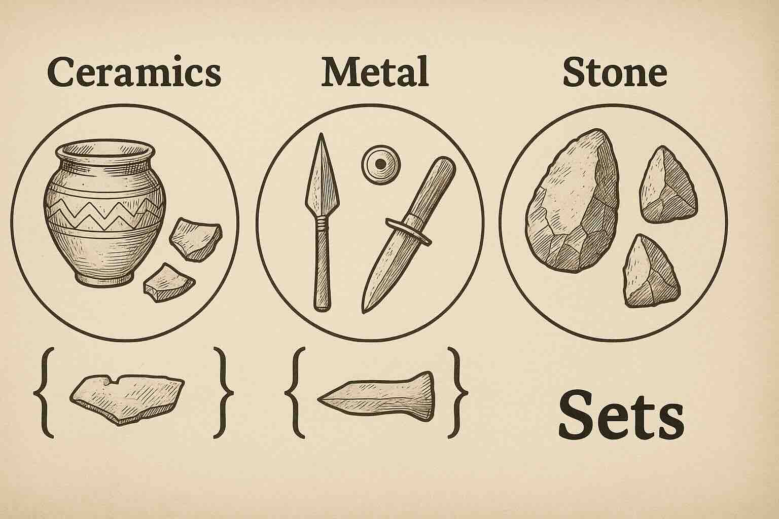
Example: A set of trench IDs where metal tools were found:

metal_trenches = {"TL01", "TL03", "TL05"}

Because sets do not allow duplicates, Python automatically ensures that each trench ID appears only once.

1.2.2 Set Operations

Python supports mathematical-style operations between sets:

  • A | B: Union — all items from both sets
  • A & B: Intersection — items common to both sets
  • A - B: Difference — items in A but not in B

Example: Let’s say we want to analyze which trenches had specific artifact types.

ceramic_trenches = {"TL01", "TL02", "TL03"}
stone_trenches = {"TL03", "TL04"}

Now apply the operations:

# Union: trenches with ceramic or stone
print(ceramic_trenches | stone_trenches)  # {'TL01', 'TL02', 'TL03', 'TL04'}

# Intersection: trenches with both
print(ceramic_trenches & stone_trenches)  # {'TL03'}

# Difference: trenches with ceramic only
print(ceramic_trenches - stone_trenches)  # {'TL01', 'TL02'}

This is useful in archaeology for comparing artifact types between excavation areas or trench phases.

1.2.3 Tuples and Lists

Tuple: Used to store fixed pairs (e.g., trench and elevation).

elevations = [("TL01", 150), ("TL02", 160)]

Each tuple is a pair where the trench ID is linked to a measurement. Tuples are immutable, meaning they cannot be changed after being created. This is useful when storing excavation records that should remain consistent.

List: A flexible structure for ordered collections.

artifact_counts = [23, 45, 12]

This could represent artifact totals found in trenches TL01, TL02, and TL03 respectively. The order matters, but you would typically store these alongside trench names using tuples or dictionaries.

1.2.4 Storing Relations as Tuples

Tuples allow us to express pairwise relationships, such as:

trench_materials = [("TL01", "metal"), ("TL02", "ceramic"), ("TL03", "stone")]

for trench, material in trench_materials:
    print(f"Trench {trench} contains {material} artifacts.")

Storing data as tuples ensures that each relationship remains tightly linked. This format mirrors rows in a spreadsheet or CSV file, making it easier to convert to a table or load into a database later.

1.2.5 Dictionaries as Functions

  • A dictionary links keys to values
  • Each key maps to one value, like a mathematical function
  • Dictionaries are fast and ideal for data lookup and mapping

Example: Trench → Artifact Count

artifact_totals = {
  "TL01": 120,
  "TL02": 85,
  "TL03": 100
}

artifact_totals["TL03"] would return 100, the number of artifacts in trench TL03. Dictionaries are very useful when your data includes labels or names and you want to retrieve associated values quickly.

You might also use dictionaries to track tool types, excavation years, or radiocarbon dates by site.

1.2.6 Nested Dictionaries for Complex Data

Most archaeologists are familiar with CSV (Comma-Separated Values) files. Here’s a basic example of how data might be structured in a CSV file:

Trench, Material, Count
TL01, ceramic, 45
TL02, metal, 30
TL03, stone, 22

This format is simple and works well for flat tables. However, archaeological data can often be hierarchical — for example, grouped by region, phase, or feature.

That’s where JSON (JavaScript Object Notation) is more powerful. JSON allows us to store nested data:

site_data = {
  "North": {"TL01": "metal", "TL02": "ceramic"},
  "South": {"TL03": "stone"}
}

This structure helps when managing multi-layered excavation units, complex features, or site-wide comparisons.

1.2.7 Choosing the Right Structure

StructureUse Case
SetTo store unique trench or artifact types
TupleFor fixed data pairs (e.g., trench and elevation)
ListTo store sequences of values with order
DictionaryFor mapping keys to values like trench to count

1.2.8 What’s Next?

In the next chapter, you’ll begin working with larger datasets — building mock excavation tables, filtering values, and loading external CSV files.

1.2.9 Quick Review

  • set(): stores unique items and supports comparisons
  • tuple: stores linked, fixed-size data pairs
  • list: stores ordered values and supports iteration
  • dict: maps labels to values for fast lookup

📘 Activity: Representing Excavation Records in Python

Scenario: You are digitizing excavation logs from Tell Logika. Your goal is to use Python to model relationships between trenches, materials, and counts.

Step-by-Step Instructions:

  1. Create a set of trench IDs where metal tools were found:
  2. metal_trenches = {"TL01", "TL03", "TL05"}
  3. Create a list of tuples representing trench IDs and elevation values:
  4. elevations = [("TL01", 150), ("TL02", 160), ("TL03", 155)]
  5. Create a dictionary mapping trench ID to artifact count:
  6. artifact_totals = {
      "TL01": 120,
      "TL02": 85,
      "TL03": 100
    }
  7. Print the total number of trenches recorded:
  8. print("Total trenches:", len(artifact_totals))
  9. Determine which trenches had both ceramic and stone artifacts using & (intersection):
  10. ceramic_trenches = {"TL01", "TL02"}
    stone_trenches = {"TL02", "TL03"}
    print("Both ceramic and stone:", ceramic_trenches & stone_trenches)

Tips for Exploration:

  • Try changing the artifact types and re-running the comparisons
  • Use print() with sorted() to see set results in order
  • Add a second level to your dictionary to include artifact type

🔗 GitHub Resources: All code and examples available here

Chapter 1.3 Structuring and Manipulating Archaeological Data

1.3 Structuring and Manipulating Archaeological Data

Objective: Build and manipulate basic datasets in Python using appropriate data structures

In this chapter, you’ll learn how to create, organize, and clean archaeological datasets using the core Python structures you’ve already explored — tuples, lists, and dictionaries. You’ll also be introduced to reading data from CSV and JSON files and preparing it for reuse or visualization.

We’ll stay at Tell Logika, our fictional excavation site, where this week’s task is to digitize and filter artifact data related to tool adoption. You’ll act as the data analyst preparing site-level data on the percentage of stone, wood, and metal tools found at various trenches.

1.3.1 What Does “Structuring Data” Mean?

  • Transforming raw information into usable formats
  • Organizing data into rows, columns, keys, and values
  • Creating predictable, searchable, and analysable structures

Unstructured data — like unlabelled field notes or inconsistent spreadsheets — is hard to work with. Structuring it gives shape to the information, allowing you to sort, filter, and analyze it computationally.

1.3.2 Mock Dataset: Lists of Tuples

Let’s say you’ve recorded tool adoption estimates at six trenches at Tell Logika:

tool_adoption = [
    ("TL01", 75),
    ("TL02", 40),
    ("TL03", 85),
    ("TL04", 20),
    ("TL05", 95),
    ("TL06", 35)
]

Each number represents the estimated percentage of metal tools versus other materials (stone or wood). This format mirrors how rows of a spreadsheet might be structured.

1.3.3 Dictionaries for Fast Lookups

tool_dict = {
    "TL01": 75,
    "TL02": 40,
    "TL03": 85
}

Dictionaries are great when you need to look up data quickly — like checking the tool adoption for trench TL03.

1.3.4 Reading Data from a CSV File

import csv

with open("tool_adoption.csv") as f:
    reader = csv.reader(f)
    for row in reader:
        print(row)

This script reads a basic CSV file. Each row might look like ["TL01", "75"]. You could then convert each row into a tuple or dictionary.

1.3.5 Reading JSON into Python

JSON (JavaScript Object Notation) is a flexible format used to store structured data, especially when it contains nesting or multiple layers (e.g., categories within sites).

{
  "TL01": {"stone": 10, "wood": 15, "metal": 75},
  "TL02": {"stone": 30, "wood": 30, "metal": 40}
}

This structure shows how JSON stores data as a dictionary, and each value can be another dictionary. This is more expressive than a CSV file, which is flat and row-based.

To read JSON in Python:

import json

with open("tool_types.json") as f:
    data = json.load(f)
    print(data["TL01"]["metal"])

This will print the percentage of metal tools in trench TL01. JSON is powerful but may be unfamiliar to many archaeologists — that’s okay! CSV is usually your starting point.

1.3.6 Cleaning and Filtering

# Filter trenches with > 50% metal tool usage
filtered = {k: v for k, v in tool_dict.items() if v > 50}
print(filtered)

You may want to isolate trenches that show early or dominant adoption of metal tools. Filtering is essential for narrowing your data focus.

1.3.7 Organizing Data for Reuse

import json

with open("filtered_tools.json", "w") as f:
    json.dump(filtered, f)

Saving data ensures you or your collaborators can reload it later for further analysis or visualization.

1.3.8 Coming Up: Visualizing Data

In Chapter 1.4, you’ll visualize this dataset using bar charts and scatterplots. You’ll explore questions like: Are metal tools more common in later trenches? Does geography influence tool type distribution?

  • Creating bar charts and scatterplots
  • Interpreting visual patterns
  • Correlating archaeological data with material transitions

1.3.9 Quick Review

  • ✅ Use tuples and lists to mock small datasets
  • ✅ Use dictionaries for quick access and lookups
  • ✅ Use csv and json for importing/exporting data
  • ✅ Filter and save cleaned data for reuse

🔍 Activity: Structuring and Filtering Tool Data from Tell Logika

Scenario: As the site data analyst, your team at Tell Logika has recorded the percentage of metal tools found in six excavation trenches. You’ve been asked to filter out only those trenches that show significant metal tool use — defined by your supervisor as greater than 50%. Your task is to build the dataset, apply this filter, and save the results for further analysis.

Instructions:

  1. Create a new folder: ComputationalArchaeology
  2. Create a subfolder: chapter1
  3. Inside it, create a Jupyter Notebook: TellLogika_Tools.ipynb

Step-by-step Python Code:

# --- CREATE DATA ---

# List of tuples (Trench ID, Metal Tool %)
tools = [
    ("TL01", 75),
    ("TL02", 40),
    ("TL03", 85),
    ("TL04", 20),
    ("TL05", 95),
    ("TL06", 35)
]

# Convert to dictionary
tool_dict = {site: percent for site, percent in tools}

print("Original Dataset:")
for site, score in tool_dict.items():
    print(f"{site}: {score}% metal tools")

print("\n---\n")

# --- FILTERING ---

# Keep only trenches above 50% metal tool usage
filtered = {k: v for k, v in tool_dict.items() if v > 50}

print("Filtered Dataset (> 50% metal tools):")
for site, score in filtered.items():
    print(f"{site}: {score}%")

# --- SAVING TO JSON ---

import json

with open("filtered_tool_sites.json", "w") as f:
    json.dump(filtered, f)

print("Filtered data saved as 'filtered_tool_sites.json'")

What This Teaches You:

  • ✅ How to represent tool-related data with tuples and dictionaries
  • ✅ How to apply filters for analytical insight
  • ✅ How to save structured data for future use

Tips for further exploration:

  • Change the filter to select trenches below 30% metal usage: if v < 30
  • Add new trenches with different values and observe how the output changes
  • Try sorting the trenches by percentage before filtering (optional challenge)
  • Modify the output format to include a summary count of high-metal trenches

Chapter 1.4 Visualizing Archaeological Data: Bar Charts and Scatterplots

1.4 Visualizing Archaeological Data: Bar Charts and Scatterplots

Objective: Learn to create basic visualizations using matplotlib and pandas

In previous chapters, you learned how to structure, filter, and clean archaeological datasets. Now, we move to the next step: making data visible. In this chapter, you’ll use Python libraries matplotlib and pandas to build simple charts that help you and others better understand patterns in archaeological data.

We continue working with our fictional excavation site, Tell Logika, where you’ll visualize metal tool adoption and compare site-level excavation data. You’ll explore how different trenches reveal different distributions when visualized as bar charts or scatterplots.

1.4.1 Why Visualize Data?

  • Visualizations reveal patterns and trends
  • They help us understand comparisons and outliers
  • Charts communicate results clearly to others

As archaeologists, we often deal with complex and layered data — counts of artifacts by type, comparisons across time periods, or material presence by site. Visualizations turn abstract data into intuitive visuals that tell a story.

1.4.2 Python Visualization Tools

  • matplotlib.pyplot: Customizable, low-level plotting tool
  • pandas.DataFrame.plot(): Simple, high-level charting using structured data

We’ll start with matplotlib to build a bar chart and scatterplot, then show how pandas simplifies charting when your data is already organized.

1.4.3 Bar Chart – Metal Tool Use by Trench

import matplotlib.pyplot as plt

metal_use = {"TL01": 75, "TL02": 40, "TL03": 85}

plt.bar(metal_use.keys(), metal_use.values())
plt.title("Metal Tool Use by Trench")
plt.xlabel("Trench ID")
plt.ylabel("% Metal Tools")
plt.grid(True)
plt.show()

Bar charts help compare categories — in this case, the percentage of metal tools found in each trench. You can immediately see which areas had higher metal adoption.

1.4.4 Scatterplot – Site Elevation vs Metal Tool Use

elevation = [150, 160, 200]  # in meters
metal_use = [40, 75, 85]
sites = ["TL02", "TL01", "TL03"]

plt.scatter(elevation, metal_use)

for i, site in enumerate(sites):
    plt.text(elevation[i], metal_use[i], site)

plt.title("Elevation vs Metal Tool Use")
plt.xlabel("Elevation (m)")
plt.ylabel("% Metal Tools")
plt.grid(True)
plt.show()

Scatterplots reveal relationships. This chart lets you ask: Do higher elevation sites show more metal tool usage? You can see this more clearly when plotted.

🔁 Try switching axes for a different perspective:

If you’d prefer to display elevation on the Y-axis (higher elevations appear higher in the chart), you can flip the axes. This helps visually emphasize elevation as a vertical dimension, which can be more intuitive.

# Flip the axes: metal use on X, elevation on Y

plt.scatter(metal_use, elevation)

for i, site in enumerate(sites):
    plt.text(metal_use[i], elevation[i], site)

plt.title("Metal Tool Use vs Elevation")
plt.xlabel("% Metal Tools")
plt.ylabel("Elevation (m)")
plt.grid(True)
plt.show()

This variation keeps the same data but shifts how we interpret it. Use whichever layout communicates your message more clearly.

1.4.5 Quick Plotting with pandas

import pandas as pd

df = pd.DataFrame({
    "Trench": ["TL01", "TL02", "TL03"],
    "Metal_Tools": [75, 40, 85]
})

df.plot(x="Trench", y="Metal_Tools", kind="bar", legend=False)
plt.title("Metal Tool Use by Trench (pandas)")
plt.ylabel("% Metal Tools")
plt.grid(True)
plt.show()

Once your data is in a DataFrame, pandas lets you create visuals with one line of code. It’s ideal for fast exploration and prototyping.

1.4.6 Basic Plot Customization

  • Add titles and axis labels
  • Use annotations to label points clearly
  • Apply gridlines for readability

Simple visual touches go a long way toward clarity. Always include titles and labels to help your viewer quickly understand your visual story.

1.4.7 Which Chart Type Should You Use?

PurposeChart Type
Compare categoriesBar chart
Show relationshipsScatterplot
Display change over timeLine chart
Show parts of a wholePie chart

1.4.8 Now It’s Your Turn!

Let’s apply your knowledge with an exercise from Tell Logika.

📊 Activity: Visualizing Tool Use at Tell Logika

Scenario: Your archaeological team has collected data on metal tool use and site elevation across three trenches at Tell Logika. You need to present this data visually to help identify patterns in metal tool distribution.

Instructions:

  1. Create a new folder: ComputationalArchaeology
  2. Create a subfolder: chapter1
  3. Create a Jupyter notebook named: Visualizing_Tools.ipynb

Use the following starter code:

import matplotlib.pyplot as plt
import pandas as pd

# Bar chart: metal use by trench
metal_use = {"TL01": 75, "TL02": 40, "TL03": 85}
plt.bar(metal_use.keys(), metal_use.values())
plt.title("Metal Tool Use by Trench")
plt.xlabel("Trench ID")
plt.ylabel("% Metal Tools")
plt.grid(True)
plt.show()

# Scatterplot: elevation vs metal use
elevation = [150, 160, 200]
metal_use = [40, 75, 85]
sites = ["TL02", "TL01", "TL03"]

plt.scatter(elevation, metal_use)
for i, site in enumerate(sites):
    plt.text(elevation[i], metal_use[i], site)
plt.title("Elevation vs Metal Tool Use")
plt.xlabel("Elevation (m)")
plt.ylabel("% Metal Tools")
plt.grid(True)
plt.show()

# pandas bar chart
df = pd.DataFrame({
    "Trench": ["TL01", "TL02", "TL03"],
    "Metal_Tools": [75, 40, 85]
})
df.plot(x="Trench", y="Metal_Tools", kind="bar", legend=False)
plt.title("Metal Tool Use by Trench (pandas)")
plt.ylabel("% Metal Tools")
plt.grid(True)
plt.show()

Tips:

  • Change trench IDs or add more data to test chart flexibility
  • Modify gridlines, labels, or chart colors
  • Use plt.savefig("filename.png") to export your charts

1.4.9 Quick Review

  • ✅ Use plt.bar() for comparing trench categories
  • ✅ Use plt.scatter() for visualizing relationships like elevation vs tool use
  • ✅ Use pandas.plot() for quick DataFrame visuals
  • ✅ Always label your axes and title your charts

Chapter 1.6: Tutorial – Excavation Insights at Tell Logika

🧭 Chapter 1.6 Tutorial: Excavation Insights at Tell Logika

Scenario:

You are part of the digital archaeology team working at the site of Tell Logika. Over the past season, you’ve collected data from multiple trenches on the percentage of metal tools found, the elevation of each trench, and the number of artifacts recovered.

Your goal is to clean, structure, analyze, and visualize this dataset to support a preliminary field report. Your team is particularly interested in identifying trenches that show early adoption of metal tools and whether elevation appears related to this pattern.


📂 Setup Instructions

  1. Open Jupyter Notebook
  2. Navigate to: ComputationalArchaeology/chapter1
  3. Create a new notebook: TellLogika_Tutorial_Summary.ipynb

🧪 Step-by-Step Instructions

✅ Step 1: Create a Structured Dataset

import pandas as pd

# Mock excavation dataset
data = {
    "Trench": ["TL01", "TL02", "TL03", "TL04", "TL05"],
    "Elevation_m": [150, 160, 200, 140, 175],
    "%Metal_Tools": [40, 75, 85, 20, 95],
    "Total_Artifacts": [120, 85, 100, 70, 140]
}

df = pd.DataFrame(data)
df

Tip: Add new trenches to test how your analysis scales.

✅ Step 2: Filter High Metal Tool Trenches

# Filter for trenches with >50% metal tools
high_metal = df[df["%Metal_Tools"] > 50]
high_metal

Try This: Change the threshold to 70% and observe the difference.

✅ Step 3: Create a Set and Explore Cardinality

high_set = set(high_metal["Trench"])
print("High Metal Trenches:", high_set)
print("Cardinality:", len(high_set))

Why: Sets help you identify unique qualifying trenches and compare groups.

✅ Step 4: Build a Lookup Dictionary

elevation_dict = dict(zip(df["Trench"], df["Elevation_m"]))
print(elevation_dict)

Try This: Access the elevation of a trench directly using its ID.

✅ Step 5: Create a Bar Chart – Metal Tool Use

import matplotlib.pyplot as plt

plt.bar(df["Trench"], df["%Metal_Tools"], color="steelblue")
plt.title("Metal Tool Use by Trench")
plt.xlabel("Trench")
plt.ylabel("% Metal Tools")
plt.grid(True)
plt.show()

Try This: Change bar color or reorder the trenches.

✅ Step 6: Create a Scatterplot – Elevation vs Metal Use

plt.scatter(df["Elevation_m"], df["%Metal_Tools"], color="darkred")

for i in range(len(df)):
    plt.text(df["Elevation_m"][i], df["%Metal_Tools"][i], df["Trench"][i])

plt.title("Elevation vs Metal Tool Use")
plt.xlabel("Elevation (m)")
plt.ylabel("% Metal Tools")
plt.grid(True)
plt.show()

Challenge: Flip the axes and visualize metal use on the X-axis.

✅ Step 7: Save a Filtered Subset

filtered = df[df["%Metal_Tools"] > 60]
filtered.to_csv("logika_high_metal_trenches.csv", index=False)

This file will appear in your Week1 folder — share it with your supervisor!


🧠 Reflection Questions

  • Which trenches had the highest proportion of metal tools?
  • Is there any visible relationship between elevation and metal use?
  • How could you extend this analysis with material type (stone, wood, metal)?
  • How did using sets and dictionaries help you organize or access the data?

🎓 What You’ve Learned (Chapters 1.1–1.4)

  • ✅ How to define and apply sets, relations, and functions
  • ✅ How to structure and filter archaeological data using lists, tuples, and dictionaries
  • ✅ How to read and clean CSV/JSON files
  • ✅ How to create and customize bar charts and scatterplots
  • ✅ How to summarize and export subsets of data for reporting

You’ve now built a complete workflow — from raw data to analysis and visualization. In the next section, you’ll test your understanding with a short quiz.

Chapter 1.7: Quiz

📊 Chapter 1.7 Self-Check Quiz: Data & Visualization Fundamentals

This interactive quiz covers key concepts from Chapters 1.1 to 1.4. After selecting your answer, immediate feedback will appear to help reinforce learning.